
While we are not sure which data analytics task is the oldest, prediction of customer churn has certainly been around for a very long time. In customer intelligence, “churn” refers to a customer who cancels a contract at the moment of renewal. A company’s CRM is often filled with such data. Identifying which customers are at risk of churning is vital for a company’s survival. Because of this, churn prediction applications are very popular, and were among the earliest data analytics applications developed.
Here we propose a classic churn prediction application. The application consists of two workflows: a training workflow (Fig. 1), in which a supervised machine learning model is trained on a set of past customers to assign a risk factor to each one and a deployment workflow (Fig. 2), in which that trained model assigns a churn risk to new customers. Both workflows are available for free download on the KNIME Hub, in the public repository Machine Learning and Marketing.
Note. More details about the repository can be found in this article: Villaroel Ordenes & R. Silipo, “Machine learning for marketing on the KNIME Hub: The development of a live repository for marketing applications”, Journal of Business Research 137(1):393-410, DOI: 10.1016/j.jbusres.2021.08.036.
Customer Data
Customer data usually include demographics (e.g. age, gender), revenues (e.g. sales volume), perceptions (e.g. brand liking), and behaviors (e.g. purchase frequency). While “demographics” and “revenues” are easy to define, the definitions of behavioral and perception variables are not always as straightforward, since both depend on the business case.
For this solution, we rely on a popular simulated telecom customer dataset, available via kaggle. In our effort to provide a broader overview of KNIME functionality, we split the dataset into a CSV file (which contains operational data, such as the number of calls, minutes spent on the phone, and relative charges) and an Excel file (which lists the contract characteristics and churn flags, such as whether a contract was terminated). Each customer can be identified by an area code and phone number. The dataset contains data for 3,333 customers, who are described through 21 features.
Preparing and Exploring the Customer Data
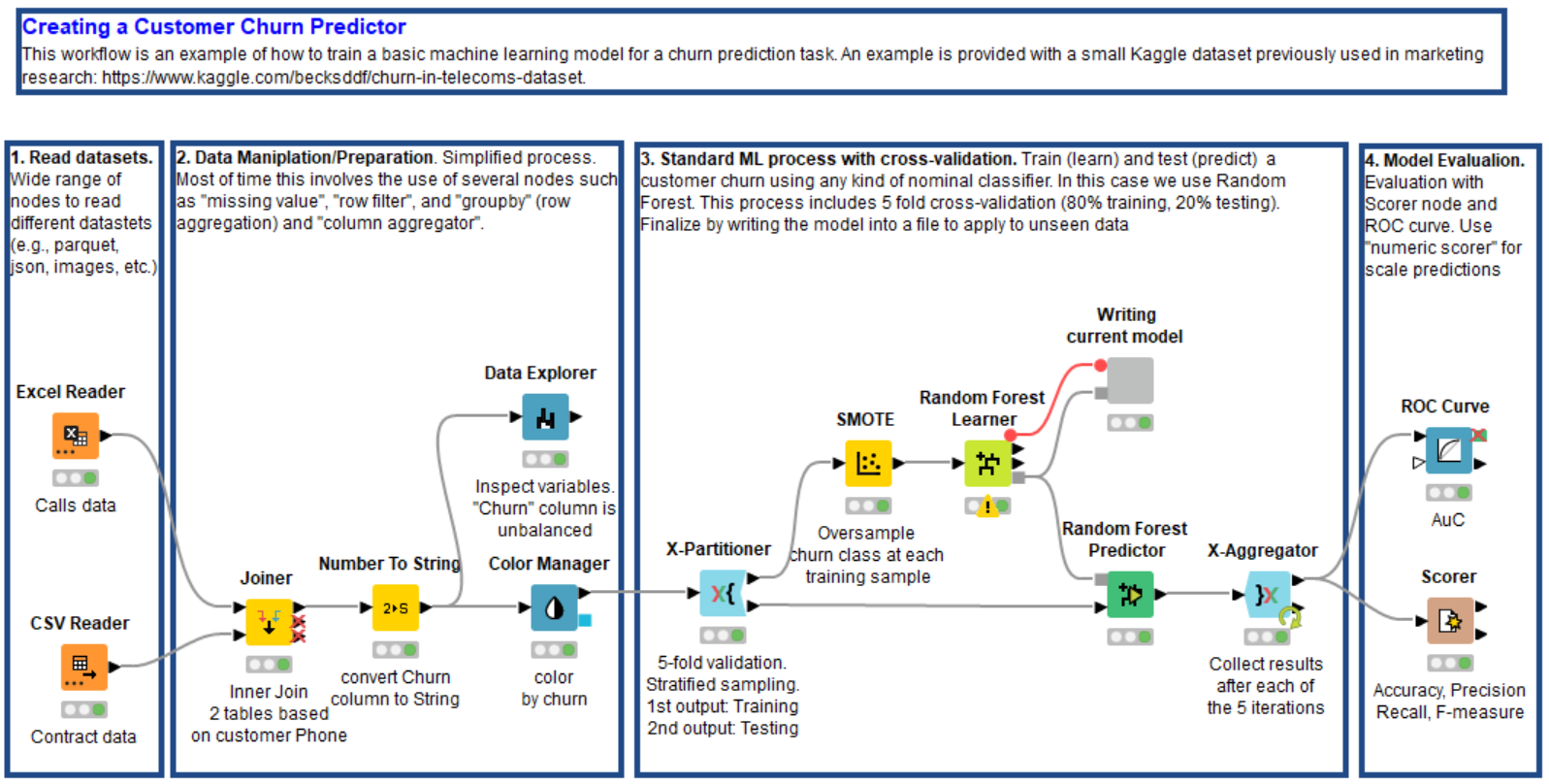
The training workflow in Fig. 1 starts by reading the data. Files with data can be dragged and dropped into the KNIME workflow. In this case we’re using XLS and CSV files, but KNIME supports almost any kind of file (e.g. parquet, json).
The second step consists of joining the data from the same customers in the two files, using their telephone numbers and area codes as keys. In the Joiner node, users can specify the type of join (inner, right, left, full).
After that the “Churn” column is converted into string type with the Number to String node to meet the requirement for the upcoming classification algorithm (in this case, nominal). Note that KNIME offers a series of nodes to manipulate data (e.g. string to date, or vice-versa).
Before continuing with further preparation steps, it is important to explore the dataset via visual plots or by calculating its basic statistics. The Data Explorer node (or else a Statistics node) calculates the average, variance, skewness, kurtosis, and other basic statistical measures, and at the same time it draws a histogram for each feature in the dataset. Opening the interactive view of the Data Explorer node reveals that the churn sample is unbalanced, and that most observations pertain to non-churning customers (over 85%), as expected. There are typically much fewer churning than non-churning customers. To address this class imbalance, we use the SMOTE node, which oversamples the minority class by creating synthetic examples. Notice that the execution of the SMOTE procedure is very time and resource consuming. It was possible here because the dataset is quite small.
Training and Testing the Customer Churn Predictor
For a classification algorithm, we chose the random forest, implemented by the Random Forest Learner node, with 5 as the minimum node size (the minimum number of observations per node) and 100 trees. The minimum node size controls the depth of the decision trees, while the number of trees controls the bias of the model. Any other machine-learning-supervised algorithm would have also worked, from one simple decision tree to a neural network. Random forest was chosen for illustrative purposes, as it offers the best compromise between complexity and performance.
A Random Forest Predictor node, which relies on the trained model to predict patterns in the testing data, follows. The predictions produced by the node will be consumed by an evaluator node, like a Scorer node or an ROC node, to estimate the quality of the trained model.
In order to increase the reliability of the model quality estimation, the whole learner-predictor block was inserted into a cross-validation loop, starting with an X-Partitioner node and ending with an X-Aggregator node. The cross-validation loop was set to run a 5-fold validation. This means it divided the dataset into five equal parts, and in each iteration it used four parts for training (80% of the data) and one part for testing (20% of the data). The X-Aggregator node collects all predictions on the test data from all five iterations.
The Scorer node matches the random forest predictions with the original churn values from the dataset and assesses model quality using evaluation metrics such as accuracy, precision, recall, F-measure, and Cohen’s Kappa. The ROC node builds and displays the ROC curve associated with the predictions and then calculates the Area under the Curve (AuC) as a metric for model quality. All these metrics range from 0 to 1; higher values indicate better models. For this example, we obtained a model with 93.8% overall accuracy and 0.89 AuC. Better predictions might be achieved by fine-tuning the settings in the Random Forest Learner node.
Deploying the Customer Churn Predictor
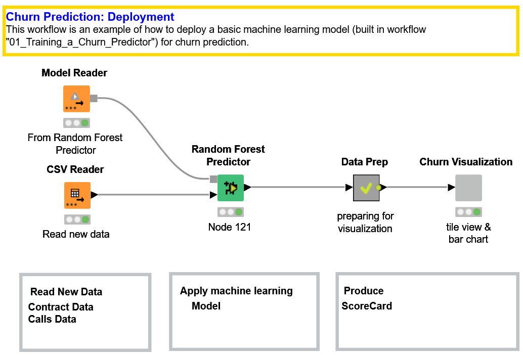
Once the model has been trained and evaluated and the researcher is satisfied with its predictive accuracy, it should be applied to new data for real churn prediction with data from the current real-world. This is the task of the deployment workflow (Fig. 3).
The best-trained model — which in this case turned out to be the one from the last cross-validation iteration — is read (Model Reader node), and data from new customers are acquired (CSV Reader node). A Random Forest Predictor node applies the trained model to the new data and produces the probability of churn and the final churn predictions for all input customers. The workflow concludes with a composite view, produced with the “Churn Visualization” component node.
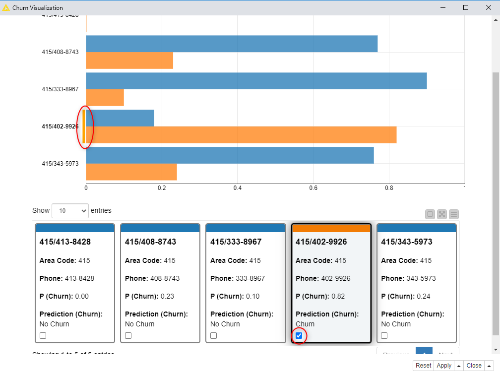
Components that contain graphical nodes inherit their interactive views and combine them into a composite view (right-click -> “Interactive View”). The composite view of the “Churn Visualization” component shows the churn risks, as bars and as tile, for the five new customers read from the CSV file. It predicts that four customers will not churn (blue), and one will (orange). All the items in a composite view are connected; selecting a tile prompts the selection of the corresponding bar in the chart, and vice-versa.
Conclusions
We have presented here one of the many possible solutions for churn prediction based on past customer data. Of course, other solutions are possible, and this one can be improved.
This particular solution included two workflows: one for training Training a Churn Predictor and one for deployment Deploying a Churn Predictor.
After oversampling the minority class (churn customers) in the training set using the SMOTE algorithm, a random forest is trained and evaluated on a 5-fold cross-validation cycle. The best trained random forest is then included in the deployment workflow.
The deployment workflow applies the trained model to the new customer data, and produces a dashboard to illustrate the churn risk for each of the input customers.