Customers who receive multiple identical emails from a company due to a data set that contains duplicates may not be pleased about this. Sending advertising letters or catalogs multiple times to identical customers is also costly. Furthermore, data deduplication in general is also very important during data preparation and preprocessing before the actual analysis and exploration.
Deduplication is the process of identifying redundant records in a data set referring to the same real-world entity and subsequently merging these together. Address data sets often contain slightly different records that represent identical addresses or names. Names of persons, streets, or cities may be written differently, are abbreviated, or misspelled. For example consider the following two addresses:
- Muller Thomas, Karl-Heinz-Ring 3, 80686, Allach
- Mueller Tomas, Karl-Heinz-Ring 3, 80686, Munich Allach
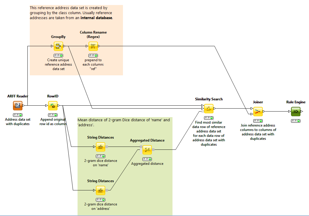
To deduplicate address data sets the records can be matched on a reference address data set in order to normalize their name and address notations.
A lot of scientific work has been done to solve this problem. The Overview of Record Linkage and Current Research Directions has detailed information to explore. In this blog article we focus on a straight forward similarity search approach in which each record of an address data set, containing duplicates is compared to representatives of groups of duplicates. These representatives can also be seen as a reference data set. The similarity or distance between address records is based on a composition of distances between multiple features, i.e. name and address.
Distance Measures and Similarity Search
The workflow illustrated in the following figure demonstrates the various possibilities of the new KNIME distance measure nodes provided since 2.10 which has been introduced in the previous blog article. A high matching accuracy is achieved with a minimum number of nodes and without any preprocessing by just aggregating distances of multiple features.
The data set we used is the "Restaurant data set" which contains 864 restaurant records and 112 duplicates. Each record consists of a name, an address, a city, a type, and a class attribute. Records with an identical class value represent the same real-word entity or restaurant in our case.
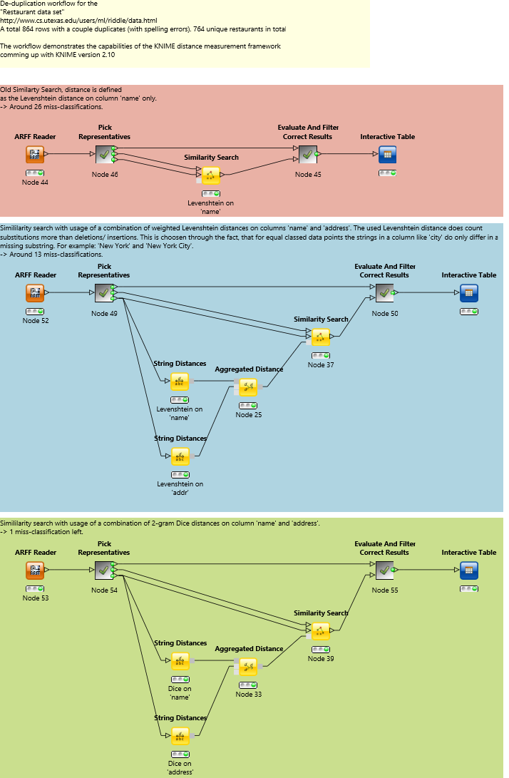
In the following we will go step by step through the workflow. It is recommended to download and import the workflow from the KNIME example server or the attachment section of this article before continuing. The workflow is split in three branches, emphasized by a red, blue and green annotation. Each of them uses a different distance measure to match the records but all of them have the same structure: The first step is to read the data, and to select the group representatives. The Pick Representatives meta node selects the first record of each class as a representative and returns them as the first and third output. The second output contains the complete data set with the original row-id appended to identify the original record later on.
In the next step the distance measure is defined and the Similarity Search node applied. The Similarity Search node assigns to each record of the query table (first input) the most similar representative of the reference table (second input). The different distance measures are described in detail below. Finally all correctly assigned records are filtered by the "Evaluate And Filter Correct Results" meta node and shown in the Interactive Table node. In the following the distance measures of the three approaches are described.
- red - regular Levenshtein distance on the name feature, leading to a misclassification rate of ~3%. But we can do better since only one attribute has been used in the distance computation.
- blue - combination of the Levenshtein distance on the name and address features. It can be seen that some address records of identical entities only differ in certain substrings e.g. "park avenue cafe" and "park avenue cafe (New York City)". With the new distance nodes we can parametrize the Levenshtein distance to take this into account. It is possible to configure the exchange operation to be more costly than insertions or deletions. With these changes we decrease the misclassification rate to ~1.5 %.
- green - combination of the N-gram Tversky distance on the name and address features. In contrast to the Levenshtein distance the N-gram Tversky distance does not rely on single operation counts, instead it models relations between neighbored letters. It outperforms the Levenshtein distance on strings which have a long identical substring. For example consider the strings "New York", "New York City" and "New Fine". Obviously the first two strings refer more to "New York" than the last one. However, the Levenshtein distance between "New York" and "New Fine" is 4 and 5 between "New York" and "New York City". The N-gram Tversky distance between "New York" and "New Fine" is 0.54 and 0.26 between "New York" and "New York City". On the other hand is the Levenshtein distance more useful on short strings containing typos, e.g. for attributes consisting of abbreviations. With this approach we end up in a misclassification rate of 0.1 % - that is only one record.
The different distance measures can be seen as models that have been learned on the training data. We can now use one of these distance measures with an appropriate clustering algorithm like the DBSCAN or Hierarchical Clustering to perform a deduplication on similar data. Furthermore it is possible to match address records on a reference data set with the customized distance measure using the Similarity Search node in order to normalize names and addresses. An example workflow is shown in the following figure and can be downloaded in the attachment section of this article.